BIOTECH-7005-BIOINF-3000
Week 11 Transcriptomics Practical - DE analysis
By Zhipeng Qu/Stevie Pederson/Jimmy Breen
- Week 11 Transcriptomics Practical - DE analysis
- Practical
Introduction
In this practical, we will be performing a Differential Gene Expression Analysis. This type of analysis compares the expression level of each gene in response to a given predictor variable (i.e. a drug-treatment), which commonly requires a control group of samples and a treated group of samples. Differential expression (DE) analysis using RNA-Seq or transcriptomes is to detect the level of activity at a genomic locus, and determine if any changes are evident due to the specific biological question.
The basic data type we work with when performing this type of analysis is a set of gene counts. These are obtained after aligning RNA-Seq reads to a reference genome, then counting how many reads align to exonic regions of each gene. As gene counts are discrete values (i.e. not continuous values) these are commonly fitted using statistical model based on Negative Binomial Models. These models can be considered as Poisson models but with the capability of handling counts which are more variable than those obtained under a strict Poisson model. Poisson models define the mean and variance of counts to be the same value, and as such, we refer to this additional variance as overdispersion.
You may also notice that each sample may have a different number of reads aligned to exonic regions, which refer to as the library size. Negative Binomial models actually analyse the rate of counts within a given library, using the size to define the rate, and an appropriate normalisation method is often required to ensure these rates capture the variability between libraries.
Whilst the statistical analysis is generally performed on the actual counts, using appropriate models, a common measurement used for visualisation is counts per millions (CPM), These are sometimes shown on the log~2~ scale, as a value referred to as logCPM. Importantly, these are most commonly just values used for visualisation, exploration and summarisation of results.
In this practical, we will be using a RNA-Seq dataset from model plant Arabidopsis thaliana to carry out a typical pairwise DE analysis.
Dataset
The dataset used in this practical is sub-sampled from RNA-Seq of two groups of samples from study of Herbst et al. 2023. We will be doing a pairwise DE analysis between Arabidopsis seedlings treated with 80 µg/ml Zeocin (treatment group) and mock-treated seedlings (control group), trying to understand what kinds of genes/pathways might be impacted by Zeocin treatment, which can be used as a radiomimetic drug to understand the molecular mechanisms of DNA damage in plants. Here are some key pieces of information for Arabidopsis and this RNA-Seq dataset:
- Reference genome build: TAIR10 (https://www.arabidopsis.org/index.jsp)
- Number of chromosomes: 5 chromosomes + Chloroplast + Mitochondria
-
Genome size: ~135 Mb
- Number of samples: 6
- Number of groups: 2, zeocin-treated and mock-treated
- Number of biological replicates per group: 3
- Sequencing type: PE150 (i.e. paired-end 150nt reads)
- Number of raw reads per sample (sub-sampled): ~2 million pairs
Tools and R packages pipeline
The pipeline of this Prac is shown in the following flowchart:
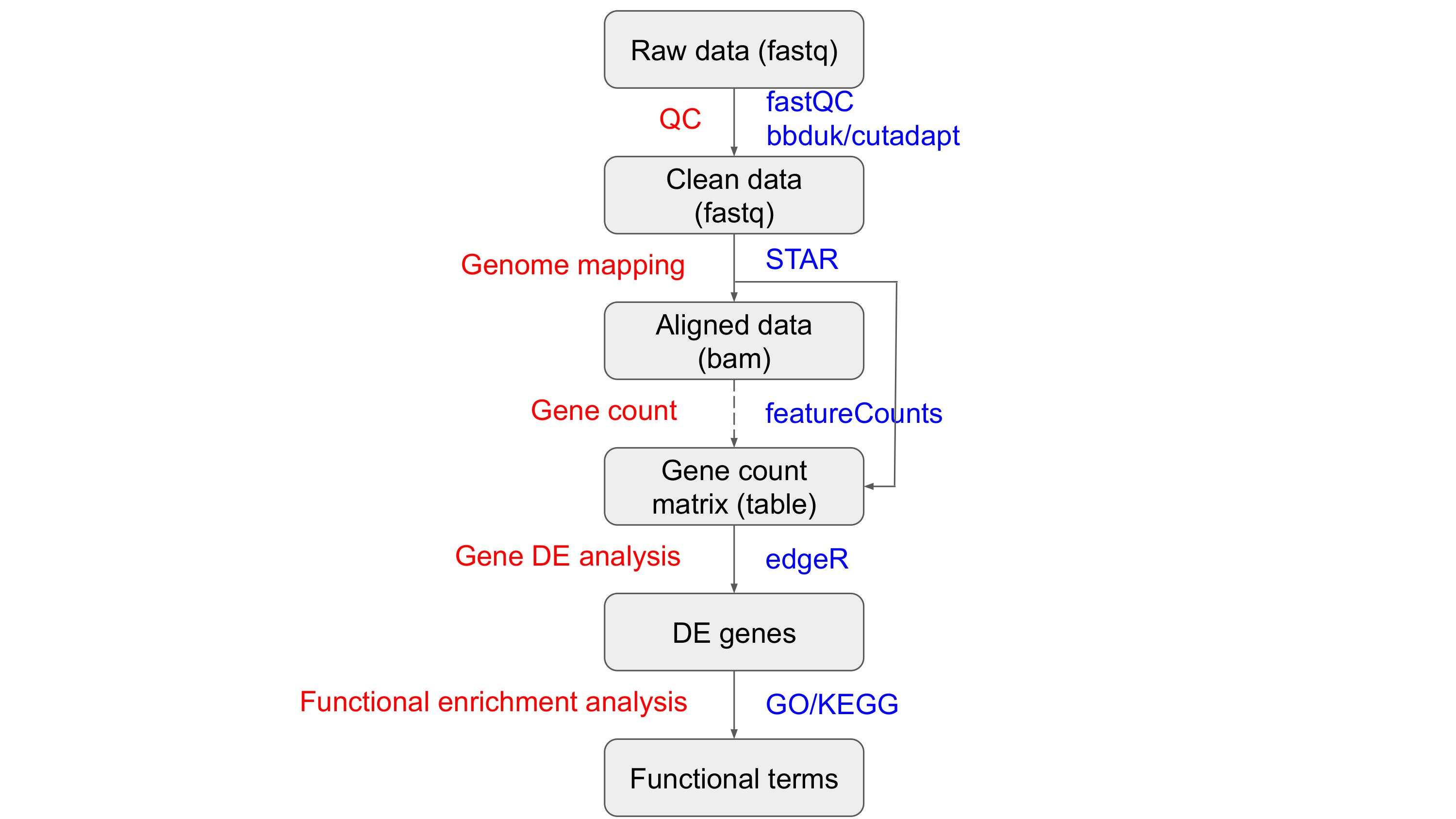
Here are some tools used in this Prac:
| Tools | Version | Link |
|---|---|---|
| fastqc | v0.11.9 | https://www.bioinformatics.babraham.ac.uk/projects/fastqc |
| bbduk | v39.01 | https://jgi.doe.gov/data-and-tools/software-tools/bbtools/bb-tools-user-guide/bbduk-guide/ |
| cutadapt | v3.5 | https://cutadapt.readthedocs.io/en/stable/ |
| STAR | v2.7.10a | https://github.com/alexdobin/STAR |
And also, we will mainly use R (4.2.2) to do DE analysis, and there is a list of R packages that we will require:
| Package | Archive | LInk |
|---|---|---|
| tidyverse | CRAN | https://www.tidyverse.org/ |
| limma | bioconductor | https://bioconductor.org/packages/release/bioc/html/limma.html |
| edgeR | bioconductor | https://bioconductor.org/packages/release/bioc/html/edgeR.html |
| reshape2 | CRAN | https://cran.r-project.org/web/packages/reshape2/index.html |
| scales | CRAN | https://scales.r-lib.org/ |
| ggplot2 | CRAN | https://ggplot2.tidyverse.org/ |
| ggsci | CRAN | https://cran.r-project.org/web/packages/ggsci/vignettes/ggsci.html |
| Glimma | biopcpnductor | https://bioconductor.org/packages/release/bioc/html/Glimma.html |
| pheatmap | CRAN | https://cran.r-project.org/web/packages/pheatmap/index.html |
Running time estimate (based on teaching VM)
The following table shows the estimated run time in VM for the major steps:
| Step | Tool/Package | Estimated run time |
|---|---|---|
| QC | fastQC | 5 mins |
| Sequence trimming | cutadapt | 10 mins |
| Genome mapping for short reads | STAR | 20 mins |
What you will learn in this Practical
- Practice bash commands you have learned
- Practice NGS QC and alignment you have learned
- Learn how to do pairwise DE analysis using RNA-Seq
Practical
There are two major steps (5 parts actually) in this Prac. Please follow the instructions in order, because some commands will rely on the results from previous commands. Please discuss the outputs and processes with the tutors/instructors to ensure everything makes logical sense to you.
Part 1. Set up and project preparation
Planning your directory structure from the beginning makes your work easier to follow for both yourself and others. This forms an important part of every transcriptomics analysis.
A common strategy is to put the initial sequencing data into a folder named data,
with the output files from different processing stages then being placed into separate folders, such as an output or a results folder.
If there are databases involved, it may be wise to create a DB folder.
Scripts may be stored in a separate scripts folder (we won’t use this folder in this Prac).
Some people also use a numbered prefix such as 01_raw_data to label different folders.
All of these naming rules are just personal preference, and feel free to build your own project folder structure rules that will help you manage large datasets
The following is the suggested folder structure for this DE analysis project:
./prac_transcriptomics_DE/
├── 01_bin
├── 02_DB
├── 03_raw_data
├── 04_results
│   ├── 01_QC
│   ├── 02_trimmed_data
│   ├── 03_aligned_data
│   └── 04_DE
└── 05_scripts
We can use following commands to build this folder structure:
cd ~/
mkdir prac_transcriptomics_DE
cd prac_transcriptomics_DE
mkdir 01_bin 02_DB 03_raw_data 04_results 05_scripts
cd 04_results
mkdir 01_QC 02_trimmed_data 03_aligned_data 04_DE
If you want to check your folder structure:
cd ~/
tree ./prac_transcriptomics_DE
Next we can build soft links of input DB and data files in our corresponding project folders:
cd ~/prac_transcriptomics_DE/02_DB
ln -s /shared/data/prac_transcriptomics_DE_data/00_DB/TAIR10_chrALL.fa ./
ln -s /shared/data/prac_transcriptomics_DE_data/00_DB/TAIR10_GFF3_genes.gtf ./
ln -s /shared/data/prac_transcriptomics_DE_data/00_DB/TAIR10_functional_descriptions.txt ./

cd ~/prac_transcriptomics_DE/03_raw_data
ln -s /shared/data/prac_transcriptomics_DE_data/01_raw_data/*.fastq.gz ./
Now all the setup work is done. Let’s move to part 2.
Part 2, QC for RNA-Seq
In this part, we will check the sequencing quality of all raw sequencing data first, and then trim adapter and low-quality sequences from raw sequencing data.
2.1 QC for illumina reads
The first step is to perform a QC analysis for the raw sequencing data using fastQC.
Check the arguments required by fastqc using fastqc --help to make sure you understand the code provided.
You can process all files all in one command:
cd ~/prac_transcriptomics_DE/04_results/01_QC
fastqc -t 2 -o ./ ~/prac_transcriptomics_DE/03_raw_data/*.fastq.gz
Or you can write a loop in your bash script to process files one by one.
After fastQC has finished running, we can check the QC report by opening the html files using web browser.
For this practical, the dataset is small enough to check QC for each file individually,
but additional tools like MultiQC can also be used to summarise QC reports across an entire dataset.
Similarly, the Bioconductor package ngsReports can be used to manually compile summary tables and figures.
2.2 Adaptor and low-quality sequence trimming
After we finish the QC for raw reads, we need to trim adapter and low-quality sequences from the raw reads.
The adapters for this RNA-Seq dataset are Illumina TrueSeq adapters as AGATCGGAAGAGCACACGTCTGAACTCCAGTCA and AGATCGGAAGAGCGTCGTGTAGGGAAAGAGTGT.
Again, check the arguments required by typing cutadapt --help or check the online manual
Following is an example commands to trim adapter and low-quality sequences for one sample, noting that we need to trim paired reads as a pair. (Ask a tutor if you’re unsure why?)
cd ~/prac_transcriptomics_DE/04_results/02_trimmed_data

# trim adaptor and low-quality sequences using cutadapt for one sample
cutadapt \
  -a AGATCGGAAGAGCACACGTCTGAACTCCAGTCA \
  -A AGATCGGAAGAGCGTCGTGTAGGGAAAGAGTGT \
  -o Col_0_mock_rep1_R1.trimmed.fastq.gz \
  -p Col_0_mock_rep1_R2.trimmed.fastq.gz \
  --minimum-length 25 \
  --quality-cutoff 20 \
  ~/prac_transcriptomics_DE/03_raw_data/Col_0_mock_rep1_R1.fastq.gz \
  ~/prac_transcriptomics_DE/03_raw_data/Col_0_mock_rep1_R2.fastq.gz
You can manually run cutadapt multiple times to trim all 6 samples, however,
the preferred way would be to write a loop in your bash script to process samples one by one.
Writing a script will also be best practice for what we refer to as reproducible research where we keep strict records of every step that we perform,
along with all tool version numbers and parameters.
This is a good moment for you to practice the skills that you learned in previous practical sessions.
(Remember to put the script that you write in the appropriate directory)
After we trim the adapter and low-quality sequences from the raw data, we have trimmed data ready for genome mapping.
Before we do the genome mapping, we can run fastQC again on the trimmed to check how we did with the trimming and to ensure that cutadapt has resolved our QC concerns.
cd ~/prac_transcriptomics_DE/04_results/02_trimmed_data
fastqc -t 2 -o ./ ~/prac_transcriptomics_DE/04_results/02_trimmed_data/*.fastq.gz
Part 3 Genome mapping/alignment
For a typical differential gene expression analysis using RNA-Seq,
we normally have the reference genome available (if you don’t have the reference genome, you can do de novo transcriptome assembly first (next Prac), and then do DE analysis based on transcriptome mapping).
We will be using a splice-aware aligner called STAR to do the genome mapping in this Prac, with the manual available here
Before we do the genome mapping, STAR requires the reference genome to be indexed.
Indexing the reference genome enables each read to be mapped to the reference by greatly speeding up the sequence searching as part of the alignment process.
We can build the Arabidopsis reference genome index using following commands:
cd ~/prac_transcriptomics_DE/02_DB
STAR \
  --runThreadN 2 \
  --runMode genomeGenerate \
  --genomeDir ~/prac_transcriptomics_DE/02_DB/TAIR10_STAR149 \
  --genomeFastaFiles TAIR10_chrALL.fa \
  --sjdbGTFfile TAIR10_GFF3_genes.gtf \
  --sjdbOverhang 149 \
  --genomeSAindexNbases 12
After we have the reference genome indexed, we can align the clean reads aginst the reference genome. The following is an example command to map one sample. Please write a loop in your bash script to process all samples.
cd ~/prac_transcriptomics_DE/04_results/03_aligned_data
STAR \
  --genomeDir ~/prac_transcriptomics_DE/02_DB/TAIR10_STAR149 \
  --readFilesIn ../02_trimmed_data/Col_0_mock_rep1_R1.trimmed.fastq.gz ../02_trimmed_data/Col_0_mock_rep1_R2.trimmed.fastq.gz \
  --readFilesCommand zcat \
  --runThreadN 2 \
  --outSAMstrandField intronMotif \
  --outSAMattributes All \
  --outFilterMismatchNoverLmax 0.03 \
  --alignIntronMax 10000 \
  --outSAMtype BAM SortedByCoordinate \
  --outFileNamePrefix Col_0_mock_rep1. \
  --quantMode GeneCounts
STAR will output multiple files with prefix Col_0_mock_rep1.
To get an idea about the mapping info, you can check Col_0_mock_rep1.final.Log.out.
Another important command option is --quantMode GeneCounts.
With this option, STAR will count number reads per gene while mapping,
and it outputs read counts per gene into a ReadsPerGene.out.tab file with 4 columns which correspond to different strandedness options:
-
column 1: gene ID
-
column 2: counts for unstranded RNA-seq
-
column 3: counts for the 1st read strand aligned with RNA (htseq-count option -s yes)
-
column 4: counts for the 2nd read strand aligned with RNA (htseq-count option -s reverse)
We will use these ReadsPerGene.out.tab files to make a gene count matrix and perform DE analysis.
The mapped reads are stored in a bam file called Col_0_mock_rep1.Aligned.sortedByCoord.out.bam.
To view this file in IGV, we need to create an index file (You can write this in the same loop as the genome mapping).
cd ~/prac_transcriptomics_DE/04_results/03_aligned_data
samtools index Col_0_mock_rep1.Aligned.sortedByCoord.out.bam
We have now finished all the steps in the first section of DE analysis, which are mainly processed using tools/commands in bash.
Next we will move to section 2, in which we will be using different R packages using RStudio.
Part 4 Gene DE analysis (under R environment)
There are multiple packages which have been developed to enable Differential Expression analysis, most of them are R-based packages.
The DE analysis in this Prac will be mainly based on the R package edgeR.
edgeR implements a range of statistical methodology based on the negative binomial distributions,
including normalisation, exact tests, generalized linear models and quasi-likelihood tests.
The original authors extend many of the approaches developed for microarray analysis in the package limma,
with the terminology tag also being used here to refer to a gene, and harking back to Serial Analysis of Gene Expression (SAGE).
If you want to understand more about edgeR,
please read one of their more recent published papers.
R environment
You should already be familiar with R/Rstudio environment by now based on what you have learned from your previous Pracs.
We have installed all required packages in your VM.
Log into your VM and open the Rstudio.
Create an R Project for This Practical
We will do the DE analysis in the folder ~/prac_transcriptomics_DE/03_results/04_DE.
Let’s make an R Project for this folder
File>New Project- Select
Existing Directory - Click the
Browsebutton - Navigate to the
~/prac_transcriptomics_DE/03_results/04_DEfolder and selectChoose - Click
Create Project
That’s everything done for the setup!!!
Load required R packages
First, we need to load all required R packages into our R workspace.
# packages for DE analysis
library(tidyverse)
library(limma)
library(edgeR)

# packages for plot
library(ggplot2)
library(ggrepel)
library(reshape2)
library(scales)
library(ggsci)
library(Glimma)

# clear workspace
rm(list = ls())

# global plot setting
theme_set(theme_bw())
Get gene annotation information
We normally want to have some additional information about the reference genes so that when we get the differential expressed genes, we can have some ideas about their functions. In this Prac, we can use following R code to get a gene annotation table for all annotated Arabidopsis reference genes.
gene_anno_df <- read.delim("/shared/data/prac_transcriptomics_DE_data/00_DB/TAIR10_functional_descriptions.txt")
gene_anno_df$Model_name <- gsub("\\..+", "", gene_anno_df$Model_name)
gene_anno_df <- gene_anno_df[!duplicated(gene_anno_df$Model_name), ]
rownames(gene_anno_df) <- gene_anno_df$Model_name
Getting the gene count matrix
The input file for our actual DE analysis will be a gene count matrix/table including the number of reads mapped to all reference genes across different groups of samples (Treatment group and control group in our dataset).
There are several tools which can be used to get gene counts based on aligned bam files from Part 3.
However, when you are using STAR to do the genome mapping, you can give parameter --quantmode GeneCounts to ensure STAR returns gene-level counts as part of the alignment process.
You may notice that when we called STAR, we didn’t provide any file that provided the gene and exon co-ordinates.
This was included in the indexing step, using the file TAIR10_GFF3_genes.gtf
# get gene count files for individual samples
star_dir <- file.path("~/prac_transcriptomics_DE/04_results/03_aligned_data")
count_files <- list.files(
  path = star_dir, pattern = "ReadsPerGene.out.tab$", full.names = TRUE
)

# create data matrix with reference genes
firstFile_df <- read.delim(count_files[1], header = FALSE)
firstFile_df <- firstFile_df[-c(1:4), ]
raw_count_mt <- matrix(0, nrow(firstFile_df), length(count_files))
rownames(raw_count_mt) <- firstFile_df[, 1]
colnames(raw_count_mt) <- rep("temp", length(count_files))

for(i in 1:length(count_files)){
  sample_name <- gsub(".+\\/", "", count_files[i])
  sample_name <- gsub("\\..+", "", sample_name)
  tmp_df <- read.delim(count_files[i], header = FALSE)
  raw_count_mt[,i] <- tmp_df[-c(1:4), 2]
  colnames(raw_count_mt)[i] <- sample_name
}

# get additional gene annotation for genes in count matrix
count_genes <- gene_anno_df[rownames(raw_count_mt),]
count_genes$gene_name <- rownames(raw_count_mt)
rownames(count_genes) <- count_genes$gene_name

# save raw count table
raw_count_df <- cbind(gene_name = rownames(raw_count_mt), raw_count_mt)
write_csv(
  as.data.frame(raw_count_df),
  file = "~/prac_transcriptomics_DE/04_results/04_DE/Table1_reference_gene_raw_count.csv"
)
In the above chunk of R code, we used a loop to merge gene count for each individual sample (ReadsPerGene.out.tab files) into one table (gene count matrix), which is required by edgeR for DE analysis.
Create DEGList objects
The type of object we will use in R for DE analysis is known as a DGEList and we’ll need to set our data up as this object type before being able to do any meaningful analysis.
# define counts, samples, groups, and gene annotation info for DEGList object
counts <- raw_count_mt
samples <- colnames(raw_count_mt)
groups <- gsub("_rep.+$", "", colnames(raw_count_mt))
genes <- count_genes

# create DEGList
dgeList<- DGEList(
  counts = raw_count_mt,
  samples = samples,
  group = groups,
  genes = count_genes
)
Notice in the $samples component, there is also a column called lib.size.
This is the total number of reads aligned to genes within each sample.
Let’s see if we have much difference between samples & groups?
dgeList$samples %>%
  rownames_to_column("sample") %>%
  ggplot(aes(x = sample, y = lib.size / 1e6, fill = group)) +
  geom_bar(stat = "identity") +
  ylab("Library size (millions)") +
  theme(axis.text.x = element_text(angle = 45, hjust = 1))
In today’s data, we don’t have a huge difference, but this can vary greatly in many experiments.
When analysing counts, the number of counts will clearly be affected by the total library size (i.e. the total number of reads counted as aligning to genes).
In some libraries, a small number of highly expressed genes can markedly inflate the library size.
Before passing this data to any statistical models, we need to calculate a scaling factor that compensates for this,
with the default approach being known as The trimmed mean of M-values normalization method (TMM),
with the full description being provided by the authors in their primary publication
dgeList <- calcNormFactors(dgeList)
Notice that now the column norm.factorsis no longer all 1.
This is used by all downstream functions in edgeR to scale the library size when fitting negative binomial models.
Data Exploration
One of the things we look for in a dataset, is that the samples from each treatment,group together when we apply dimensional reduction techniques such as Principal Component Analysis (PCA) or Multi Dimensional Scaling (MDS).
The package edgeR comes with a convenient function to allow this.
cols <- pal_npg("nrc", alpha=1)(2)

plotMDS(dgeList, labels = dgeList$samples$type, col = cols[dgeList$samples$group])
Here we can see a clear pattern of separation between the groups.
(If we don’t see this, it may mean we have some difficult decisions to make. Maybe we need to check our samples for mislabelling? Maybe there is some other experimental factor which we’re unaware of.)
An interesting way to view our data is to use the value known as Counts per million.
This accounts for difference in library sizes and gives an estimate of how abundant each gene is.
head(cpm(dgeList))
You can see from this first 6 genes, that we have one highly abundant gene, and a couple with far lower expression levels.
Removing ‘undetectable’ genes
Genes with low count numbers give us minimal statistical power to detect an changes in expression level, so a common approach is to filter out these genes. This reduces the issues which we will face due to multiple hypothesis testing, effectively increasing the statistical power of a study. We often refer to this as removing undetectable genes, although we will discard some genes with very low counts.
A common method would be to remove any genes which are below a specific CPM threshold in the majority of samples. In this dataset, we might like to remove genes which have $<1$ CPM in 4 or more samples. For a dataset with an average library size of 20m reads, this roughly equates to 20 counts, but using CPM allows for significant varibility in library sizes.
Any number of strategies can be applied for this stage.
We can plot the densities of each of our samples using log-transformed CPM values, and the clear peak in the range of very low expression is clearly visible.
plotDensities(cpm(dgeList, log = TRUE), main = "all genes", legend = "topright")
Let’s filter our dataset, and remove genes with low signal.
genes2keep <- rowSums(cpm(dgeList) > 1) > 3
Here we’ve created a logical vector defining which genes to keep. To get a quick summary of this enter
summary(genes2keep)
Now let’s look at the densities after filtering. Notice how all of the genes with low signal (at the LHS of the original plot) are no longer included and only the secondary peak, corresponding to higher signal (or detected) genes is retained.
plotDensities(cpm(dgeList, log = TRUE)[genes2keep, ], main = "fitered genes", legend = "topright")
Now we’re happy that we have the genes we can extract meaningful results from, let’s remove them from our dataset.
dgeList <- dgeList[genes2keep, ]
Calculating moderated dispersions
Most RNA-Seq analysis is performed using the Negative Binomial Distribution. This is similar to a Poisson distribution, where we count the number of times something appears in a given interval. The difference with a Negative Binomial approach is that we can model data which is more variable. Under the Poisson assumptions, the variance equals the mean, whilst under the NB this is no longer required.
This extra variability is known as the dispersion, and our estimates of dispersion will be too high for some genes, and too low for others. Taking advantage of the large numbers of genes in an experiment, we can shrink the ones that are too high, and increase the ones that are too small. This is an important step in RNA Seq analysis, as it reduces the number of false positives, and increase the numbers of true positives.
Before we do this, we need to define our statistical model.
Here, our term of interest is in the column group, and we’re using R’s formula notation ~ group.
This can be read as depends on group, where the dependent variable is not defined, but can be considered to be the gene expression values for all genes.
design <- model.matrix(~ group, data = dgeList$samples)
design
dgeList <- estimateDisp(dgeList, design = design)
Performing differential expression analysis
The most common analytic approach we use is the Quasi-Likelihood approach to the Generalised Linear Model used to fit Negative Binomially distributed data.
In the following line of code, we are comparing the first two groups in our data. Clearly we only have two groups in this dataset,but it is quite common to have multiple groups in other analyses.
fit <- glmQLFit(dgeList)
This simply fits the model without the final step of testing for significance.
The full table of results can be returned using the Quasi-Likelihood F-Test,
then using some tidyverse skills to extract the topTags() (i.e. genes) and return a tibble
results <- glmQLFTest(fit)
topTable <- results %>%
  topTags(n = Inf) %>%
  pluck("table") %>%
  as_tibble()
Find the highest ranked gene in this dataset If it’s been given a negative value for logFC, this means lower expression is likely to be observed in the second of the two conditions. The opposite is true for a positive value for logFC. Let’s check the raw counts using logCPM
cpm(dgeList, log= TRUE)["AT5G48720",]
Inspect a few more of the highly ranked genes, so make sure you can understand these results.
Let’s get a list of significant genes, by using an FDR of 0.01.
sigGenes <- filter(topTable, FDR < 0.01)$gene_name
And we can check the number of significant genes
length(sigGenes)
We can save the statistically significant DE genes into a table for future downstream analysis
topTable %>%
  dplyr::filter(FDR < 0.01) %>%
  write_csv(
    "~/prac_transcriptomics_DE/04_results/04_DE/Table2_sigGenes.csv"
  )
Now we can visualise the pattern of logFC to expression level. We can use plotMD to generate MD (mean-difference) plot showing the library size-adjusted log-fold change between two libraries (the difference) against the average log-expression across those libraries (the mean). We can use the following command to compare sample 1 (Col_0_mock_rep1) to an artificial reference library constructed from the average of all other samples.
plotMD(dgeList, status = rownames(dgeList) %in% sigGenes, column = 1)
An alternative is to plot the logFC in relation to the $p$-value, to make what is known as a volcano plot.
topTable %>%
  mutate(DE = Geneid %in% sigGenes) %>%
  ggplot(aes(x = logFC, y = -log10(PValue),colour = DE)) +
  geom_point() +
  scale_colour_manual(values = c("grey50", "red"))
We can also generate interactive HTML graphics to examine the expression difference of individual genes between groups using R package Glimma.
glMDPlot(
  results,
  counts = cpm(dgeList, log = TRUE),
  groups = dgeList$samples$group,
  status = results$FDR < 0.01,
  main="MD plot: Col_0_Zeocin_vs_Col_0_mock",
  side.main = "ID",
  side.ylab = "Expression (logCPM)",
  sample.cols = pal_npg()(2)[dgeList$samples$group],
  folder = "glimma_plot",
  launch = FALSE
)
Part 5 Additional analysis
After we get a list of DE genes between groups (e.g. treatment group vs control group in our dataset), we can do all different kinds downstream analyses based on this DE gene list. One common downstream analysis is the functional enrichment/over-representation analysis.
There are many tools/packages which can be used to do functional enrichment analysis for DE genes. One popular and easy-to use tool is the web-based DAVID (Database for Annotation, Visualization and Integrated Discovery). The question we’ll ask using this tool is to see which gene-sets or pathways appear in our set of DE genes more often than we might expect. This requires a set of background (i.e. not DE) genes, and using the background genes we can determine of a pathway is enriched amongst the DE genes.
See if you can find your way around the DAVID interface and ask for help if the questions the tool asks are confusing.