BIOINF-3010-7150
Graph Genomes Practical: Part 2
By Chelsea Matthews - modified from Yassine Souilmi
Learning Outcomes
-
Have a basic understanding of genotyping and how we can extract variants from a graph constructed from a Multiple Sequence alignment.
-
See how alignment parameters (in this case minimum read length match) can alter alignment rates.
-
See how read alignment rates to a linear reference compare with alignment rates to a graph incorporating variants found within that population.
Getting (re)started
Let’s load the tools we’ll need today.
source activate bioinf
The tools we’ll need today include:
vg
bcftools
jq -h
dot --help
You’re already familiar with vg and dot from the first practical.
You may have used bcftools before but if not, it’s a tool that is designed for use in variant calling pipelines.
It allows us to manipulate VCF (variant call format) files which is what we’ll use it for today.
And finally, jq.
This is a tool for processing and filtering JSON files.
We will be using it, as well as a few other commands, to summarise read alignment rates against different graphs.
We’ll create a new directory for todays prac so we don’t get too confused by all the files.
Copy all of the files from data/graph_genomes/prac2/ into a new directory for todays practical.
cd into that directory.
cd ~
mkdir -p GraphGenomes/prac2/{yeti,cannabis,1000genomes}
cp /shared/data/Graph_Genomes/prac2/{z.*,README.md} ~/GraphGenomes/prac2/1000genomes/.
cp /shared/data/Graph_Genomes/prac2/{yeti*,nylamo*} ~/GraphGenomes/prac2/yeti/.
cp /shared/data/Graph_Genomes/prac1/cannabis.fasta ~/GraphGenomes/prac2/cannabis/.
cd ~/GraphGenomes/prac2
You should get the following by running tree from the GraphGenomes/prac2 diretory.
.
├── 1000genomes
│   ├── README.md
│   ├── z.fa
│   ├── z.fa.fai
│   ├── z.vcf.gz
│   └── z.vcf.gz.tbi
├── cannabis
│   └── cannabis.fasta
└── yeti
    ├── nylamo.fq
    ├── yeti.fa
    └── yeti.vcf
Part 1: Variant Calling and Inference
Part 1.1: Infer variants from an MSA graph - Cannabis dataset
In the last practical we constructed a graph using the multiple sequence alignment technique for 4 different cannabis sequences from the same region of the genome and looked at the differences in their structure using visualisation techniques. We will now use this same graph but will call variants from the graph programmatically.
Let’s build the graph again.
Move into the cannabis directory, construct the graph, and index it (we only need the xg index).
cd ~/GraphGenomes/prac2/cannabis
vg msga -f cannabis.fasta -t 2 -k 16 --base pink_pepper | vg mod -U 10 - | vg mod -c -X 256 - > cannabis.vg
vg index -x cannabis.xg cannabis.vg
It’s exactly the same graph as we used in the first part of the practical and we are interested in the regions circled below.
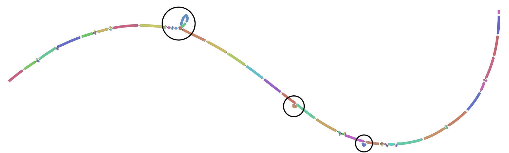
Now use vg deconstruct to generate a VCF using the pink_pepper sequence as the reference.
Notice how deconstruct is the opposite to construct?
We use the vg construct command to build a graph with a reference and a set of variants, and we use the vg deconstruct command to extract variants from a graph.
vg deconstruct cannabis.xg -e -p "pink_pepper" > variants.vcf
Let’s have a look at the resulting file.
less variants.vcf
Unfortunately the vcf’s produced by vg don’t give us the type of variant or its length but I think we can work it out.
- What are the positions of the three structural variants we looked for last time (duplication, insertion, and deletion)?
This method is obviously much easier than manually looking through a graph to work out how each sample varies from the reference and can be used at much larger scales than we have just seen.
Part 1.2: Genotyping and Variant Discovery - Yeti dataset
Now let’s explore how read alignment to a graph can be used to genotype a newly sequenced sample.
Genotyping is where we identify the specific genomic makeup of a sample. In this case, we will use a graph constructed from known variants found within a particualr population and we will identify which of these variants a newly sequenced sample has. This process is used for a range of applications. For example, genetic screening. If we know of the specific variants that cause certain diseases, we can use genotyping to determine whether a person/organism will have those diseases or not.
You have been provided with a yeti reference sequence yeti.fa and a vcf - yeti.vcf.
The vcf contains variants called from a number of different types of yeti’s and so should hopefully represent a good range of the natural genomic variation within the yeti population.
There are also reads in a file called nylamo.fq.
Nylamo is the yeti sample that we will be genotyping.
First, we build a variant graph from the reference genome and the vcf.
Note that unlike in prac 1, we must include the -a option in our vg construct call.
cd ~/GraphGenomes/prac2/yeti
vg construct -r yeti.fa -v yeti.vcf -a > yeti.vg
- Can you tell what the
-aoption does?
Index this graph as below and then have a quick look at it. Again note that the xg indexing command is slightly different.
vg index -x yeti.xg -L yeti.vg
vg index -g yeti.gcsa -k 16 yeti.vg

vg view -dpn yeti.vg | dot -Tpdf -o img_yeti_dot.pdf
vg view yeti.vg > yeti.gfa
Bandage image yeti.gfa img_yeti_bandage.png
Align the reads in nylamo.fq to the graph.
vg map --fastq nylamo.fq -x yeti.xg -g yeti.gcsa > nylamo.gam
Now, we will now use vg pack to determine read support for the graph.
vg pack -x yeti.xg -g nylamo.gam -o nylamo.pack
And finally, we will genotype the sample.
vg call yeti.xg -k nylamo.pack -v yeti.vcf > nylamo_genotype.vcf
Open the output file so that you can have a look at it.
The genotype of the sample is found at the start of the final column. For example, 0/0 means that the sample was homozygous for the reference allele. 1/1 indicates that the sample is homozygous for the alternative allele. 1/0 means that the sample was heterozygous with one copy of the reference allele and one copy of the alternate allele
Questions:
- Which variants are present in the nylamo sample? Which variants are not?
- Can you find the quality scores and read depth for each variant call?
- Why might using a graph for variant calling be better than using a linear reference genome?
Part 2: Investigating factors impacting read alignment to graphs
Let’s move on to the 1000 Genomes data.
cd ~/GraphGenomes/prac2/1000genomes
The z files contain 1Mbp of 1000 Genomes data for chr20:1000000-2000000.
The reference sequence is contained in z.fa, and the variation is contained in z.vcf.gz.
Background and Setup
The goal of this section is for you to investigate how read alignment rates change with one of two conditions but before you split off to investigate on your own, we will go through the setup and the questions.
We will initially build two graphs - one with just the reference sequence and one with variation obtained from the 1000 Genomes project.
Take a look at the data first.
gunzip -c z.vcf.gz | less
- Build a reference-only graph named
ref.vg - Build the same graph but with variation included named
z.vg
vg construct -r z.fa -m 32 > ref.vg
vg construct -r z.fa -v z.vcf.gz -m 32 > z.vg
You might be tempted to visualize these graphs (and of course you are welcome to try), but they are sufficiently big already that your machine might run out of memory and crash.
Now index your graphs.
In a nutshell, mapping reads to a graph is done in two stages: first, seed hits are identified and then a sequence-to-graph alignment is performed for each individual read. Seed finding hence allows vg to spot candidate regions in the graph to which a given read can map potentially map to.
vg index -x z.xg z.vg
vg index -g z.gcsa z.vg
vg index -x ref.xg ref.vg
vg index -g ref.gcsa ref.vg
We will now simulate some reads from our graph.
The -a parameter tells vg to output the read as well as information describing exactly where that read came from in the graph and hence, exactly where it should align to the graph when we map our reads.
Keep in mind that this information is only relevant if we are mapping reads back to the exact same graph they were generated from.
This information will be needed if you choose Option 1 but Option 2 also requires simulated reads and this format is fine so we can make them together.
vg sim -x z.xg -l 100 -n 1000 -e 0.01 -i 0.005 -a > z.sim
- What do these reads actually represent?
Now let’s map these reads to our graph and find out how the alignment went.
Map using the command below and then take a look at the aln_sum.json
The -j parameter outputs a JSON file describing how each read mapped to the graph and how this compares with its true location.
vg map -x z.xg -g z.gcsa -G z.sim --compare -j | head -n 1
The above command should have printed a chunk of text to your terminal that describes how just one of your reads aligned to the graph.
- Can you understand it?
As you can see, there’s way too much information for us to go through manually.
We can process ths information with jq, awk, and sed to get a summary of alignment correctness.
We can use this to quickly check if our alignment process is doing what we expect on the variation graph we’re working on.
For instance, we might have set alignment parameters that cause problems for our alignment which we could observe using the --compare feature of the mapper.
Let’s summarise the alignment correctness for the mapping we just did but keep in mind that your results will be slightly different from mine because we all have a slightly different set of reads and also, the alignments may come out in a different order over multiple runs.
vg map -x z.xg -g z.gcsa -G z.sim --compare -j | jq .correct | sed s/null/0/ | awk '{i+=$1; n+=1} END {print i/n}'
Questions:
- What is the
jq .correctpart doing? - What is the
sedpart doing? - What is the
awkpart doing? - How well were our reads aligned? Why isn’t this number 1?
- What might we put instead of
jq .correctto get some idea of how well our reads aligned to a graph they didn’t come from?
The goal of this final section is for you to investigate one (or both) of the following questions on your own or in a group using the method above to summarise read alignment correctness or read identity if you’re choose option 2.
Option 1:
- How does the minimum Maximal Exact Match (MEM) length impact read alignment rates and accuracy?
Option 2:
- How do read alignment rates and accuracy compare when using a linear reference, a graph containing only common variants, and a graph containing all variants for that population?
Option 1 Instructions
The -k parameter used when mapping reads to a graph is described as “minimum MEM length” in the documentation.
MEM stands for “Maximal Exact Match”.
MEM’s are exact matches between two sequences that cannot be extended either way without introducing even one mismatch.
They are used in read alignment as “seeds”, possible locations that the read could align.
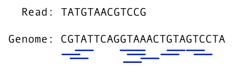
The figure below shows all of the Maximal Exact Matches between a read and a genome for a value of k=3, meaning that the length of matching sequences found in both the read and the genome will be 3 or more. Therefore, all k-mers of 3 or more basepairs common to both the read and the reference are underlined. These matches are used as starting points, or “seeds”, for read alignment.
You can vary this parameter within the mapping command by changing the question mark below to your k-value of choice.
vg map -k ? -x z.xg -g z.gcsa -G z.sim --compare -j | jq .correct | sed s/null/0/ | awk '{i+=$1; n+=1} END {print i/n}'
Questions:
- Does read alignment correctness get better or worse as k increases?
- For what (approximate) range of k values does read alignment correctness remain the same? Can you explain why?
- If our reads had a higher error rate, would this range of k values change? How?
- Would it be sensible to choose a very small value of k (eg
-k 5) as a default value? Why or why not?
Option 2 Instructions
You are investigating how read alignment rates change with the amount of variation within a graph.
We have already built a graph with no variation - ref.vg, and a graph with all of the variants identified in the 1000 genomes project for this section of the genome - z.vg
You will now build a graph containing only variants found within at least 20% of the population and compare read alignment rates between the three graphs.
You can make a VCF with a minimum allele fequency with the command below noting that AF stands for allele frequency:
bcftools filter -i 'AF > 0.2' z.vcf.gz > af20.vcf
Next, build a new graph using the reference and this filtered VCF.
vg construct -r z.fa -v af20.vcf -m 32 > af20.vg
vg index -x af20.xg af20.vg
vg index -g af20.gcsa af20.vg
You should now have three graphs:
ref.vg - just the reference sequence, no variation
20af.vg - graph containing common alleles only
z.vg - graph containing all alleles identified in the 1000 genomes project for this section of the genome
Now, align your simulated reads to all three graphs one at a time and compare mapping identity rates.
We don’t have a “truth set” for the alignment of these reads to either the ref.vg or filtered.vg graphs because they didn’t originage from either of these graphs.
Therefore, when we filter using jq, we will use .identity instead of .correct.
For example, the command to align to z.vg and summarise read mapping identity would be:
vg map -x z.xg -g z.gcsa -G z.sim --compare -j | jq .identity | sed s/null/0/ | awk '{i+=$1; n+=1} END {print i/n}'
Feel free to build another graph with a different allele frequency cutoff to explore further.
Questions:
- What was the read alignment identity for each of your graphs?
- Take a look at the file sizes for each of your .vg graphs and their .gcsa index. How do these files scale with the amount of variation within the graph?
- Given that the .gcsa index is a k-mer index that is used for read alignment, how might the addition of a single variant to the graph alter the number of k-mers in the graph? It might help to draw a picture.
Summary
- Using a pan-genome graph in the place of a linear reference genome reduces reference bias
- By incorporating variation into a graph, we improve read alignment rates, and improve our ability to find new variants
- Using a graph in place of a linear reference is complex and methods are still under development