BIOINF-3010-7150
SAMtools and alignments practical : Part 1
By Jimmy Breen, updated/adapted by Dave Adelson
- SAMtools and alignments practical : Part 1
- By Jimmy Breen, updated/adapted by Dave Adelson
- Practical Outcomes
- Before high-throughput sequencing: Why do we need a format to store alignments?
- CRAM, BAM and SAM
- Today’s data
- File sizes
- Viewing alignments
- Summary statistics
- Headers
- Filtering an alignment file
- Mapping Quality (MAPQ)
- Assessment of alignment rate and multi-mapping
- To deduplicate or not to deduplicate? That is the question
- Evaluate with and without
- What does coverage look like?
- How do we look at our alignment?
- To save space once you are done with practical, you should delete
SRR3096662_Aligned.out.sort.cram,GRCh37.p13.genome.fa.gzandSRR3096662.tar.gz
Fundamental to the analysis of genomic data is the availablility, or lack there of, of a reference sequence. The reference sequence gives a substrate to compare to and is critical for many routine Bioinformatics tasks. In alignment tasks, sequenced DNA fragments (or “reads”) are matched to the reference sequence in a process called “Alignment”.
Today we are not going into the details of the alignment process, but will get stuck into some common commands and processes that will enable you to assess the quality of your alignments.
Practical Outcomes
- Learn what an alignment file is; i.e. SAM, BAM and CRAM files
- Run commands that help you view and produce statistics on the quality of alignment files
- Establish how to filter alignments
- Visualise alignment coverage, and investigate the patterns that different genomics applications make when aligning over the reference sequence
Before high-throughput sequencing: Why do we need a format to store alignments?
While many modern genome sequences were produced at the start of the 21st century, sequencing machines were limited in their throughput i.e. the number of DNA fragments that could be sequenced at one time. Bioinformatics and genomics analyses during this time centred mainly on sequence searching with local alignment tools such as the very popular Basic Local Alignment Search Tool (BLAST). BLAST is one of the most widely used computational tools in biological research, and two versions of the program are the 12th and 14th most cited research publications of ALL TIME.
Local alignment works by matching substrings of a sequence to a reference database, which is computationally intensive when scaling to large numbers of sequence searches. As high-throughput sequencing machines were further developed in the late 2010s, global or “end-to-end” alignments offered a faster and more appropriate way of identifying the position of a DNA fragment if the sample was close to the appropriate reference sequence.
So how do you store alignment information for each DNA fragment? In 2009, Bioinformaticians at some of the major DNA sequencing institutions at the time, namely the Sanger Institute (UK) and the Broad Institute (Boston, USA), developed a format to store information about where a sequence read aligned to the reference, and importantly, how uniquely it aligned to the identified region.
CRAM, BAM and SAM
SAM, BAM and CRAM are all different forms of the original SAM format that was defined for holding aligned (or more properly, mapped) high-throughput sequencing data. SAM stands for Sequence Alignment Map, as described in the standard specification, and was designed to scale to large numbers of reads sequenced at a given time.
The basic structure of the SAM format is depicted in the figure below:

SAM files contain a lot of information, with information for every mapped fragment (and sometimes unmapped sequences) being detailed on a single line of text. Text data generally takes up a large amount of storage space, meaning SAM files are an inefficiant storage format for alignment data. Instead, storage formats such as BAM and CRAM are often favoured over SAM as they represent the alignment information in a compressed form. BAM (for Binary Alignment Map) is a lossless compression while CRAM can range from lossless to lossy depending on how much compression you want to achieve (up to very much indeed). Lossless means that we can completely recover all the data when converting between compression levels, while lossy removes a part of the data that cannot be recovered when converting back to its uncompressed state. BAMs and CRAMs hold the same information as their SAM equivalent, structured in the same way, however what is different between them is how the files themselves are encoded.
While numbers may vary, generally the file compression that can be achieved from converting the text rich SAM file into the binary BAM version is 1 in 8/10.
Using the default lossless compression in samtools (which we will use below), we can almost half the size of a BAM file when converting to a CRAM file.

Most analysis programs that deal with alignments will take SAM and BAM files as input and/or output, and the majority will strictly ask for BAMs as they are more compressed than SAMs. CRAM files are increasing in popularity and can generally be used with most major programs, with older version containing more limited options for CRAM input.
Additional info
Aaron Quinlan (University of Utah) has a really nice presentation that goes through a lot of the things we’ll be going through today.
Today’s data
The CRAM file that we will be using today is an alignment produced from the alignment of RNA sequencing reads to the human reference genome version 19, or GRCh37. You can download the reference genome sequence and gene annotation from this version at GENCODE. The sample itself is taken from the Chorionic Villus of a human placenta as part of the Rhode Island Child Health Study (RICHS), which enrolled a total of 899 mother/infant pairs at Woman and Infant’s Hospital of Rhode Island (Providence, RI, USA). This particular placenta was taken from the placenta of a healthy female that was born >37 weeks gestational age (a full term). Full public information of this sample is available at the NCBI Short Read Archive (SRA).
You will find the data in ~/data/SAM_prac in your home directory .
To obtain the files:
cd

#make practical directories
mkdir -p ./Project_2/data

#copy data to todays's practical directory
cp ./data/SAM_prac/* ./Project_2/data/

cd ~/Project_2/data

#decompress files (this may take 2-3 minutes)
tar -xvf SRR3096662.tar.gz

#have a look at what the result of the previous command is
ls -lrth

cd ../Project_2
File sizes
As mentioned above, the size differences between SAM, BAM and CRAM files can be surprising.
From today’s CRAM file, the converted SAM and BAM files are much larger in size. While we have not included the original SAM file as it is very large, here is a comparison of the file sizes, including the human readable .sam file.
37G SRR3096662_Aligned.out.sort.sam
~3G SRR3096662_Aligned.out.sort.bam
1.56G SRR3096662_Aligned.out.sort.cram
A 37GB SAM file can be compressed into a 2.8GB BAM file and 1.5GB CRAM file! Today’s practical includes a BAM and CRAM file, but not the SAM file in order to save time copying/accessing data.
Viewing alignments
To view a SAM, CRAM or BAM file, you can use the program samtools.
samtools is a very common tool in Bioinformatics and we will be using it frequently in this course.
Lets quickly view our file using the samtools view subcommand, which is similar to the command-line tool cat in which the file is read to our screen line by line. Make sure you are in your Project_2 directory.
samtools view ./data/SRR3096662_Aligned.out.sort.bam
As you can probably see, there is a lot of data flashing on your screen.
You can interupt this stream by using/pressing Ctrl + C a few times, which should cancel the command.
What you just saw was the alignment information for each read in the SRR3096662 sample.
Lets use the pipe (|) and head command to just give us the first five lines of the file so we can start to make sense of the file format.
samtools view ./data/SRR3096662_Aligned.out.sort.bam | head -n5

SRR3096662.22171880 163 1 11680 3 125M = 11681 126 CTGGAGATTCTTATTAGTGATTTGGGCTTGGGCCTGGCCATGTGTATTTTTTTAAATTTCCACTGATGATTTTGCTGCATGGCCGGTGTTGAGAATGACTGCGCAAATTTGCCGGATTTCCTTTG BBBBFFFFFFFFFFFFFFFFFFFFFFFFFFFFFFFFFFFFFFFFFFFFFFFBFFFFFFFFFFFFFFFFFFFFBF<FFFFFFFFFFFFFFFFFFFFFFFFFFFFFFFFFFFFFFFFFFFFFBFFFF NH:i:2 HI:i:1 AS:i:244 nM:i:2 MD:Z:28G96 NM:i:1 RG:Z:SRR3096662
SRR3096662.22171880 83 1 11681 3 125M = 11680 -126 TGGAGATTCTTATTAGTGATTTGGGCTTGGGCCTGGCCATGTGTATTTTTTTAAATTTCCACTGATGATTTTGCTGCATGGCCGGTGTTGAGAATGACTGCGCAAATTTGCCGGATTTCCTTTGC FFF<FFFFFFFFFFFFFFFFFFFFFFFFFFFFFFFF<FFFFFFFFFFFFFFFFFFFFFFFFFFFFFFFFFFFFFFFFFFFFFFFFFFFFFFFFFFFFFFFFFFFFFBFFFFFFFFFFFFFFBBBB NH:i:2 HI:i:1 AS:i:244 nM:i:2 MD:Z:27G97 NM:i:1 RG:Z:SRR3096662
SRR3096662.15588756 419 1 12009 0 10S115M = 12048 164 GCTTGCTCACGGTGTCTGACTTCCAGCAACTGCTGGCCTGTGCCAGGGTGCAAGCTGAGCACTGGAGTGGAGTTTTCCTGTGGAGAGGAGCCATGCCTAGAGTGGGATGGGCCGTTGTTCATCTT BBBBFBFBFFFFFFFFFFFFFFBFFFFFFFFF/FFFFBFFFFFFBB</BF<FFFFFFFFFFFFFFFF/<FFF<FFFFB<FBFB<F/BFFFFBFFBFFFFFBFBFFFFFFFFFFFFFFFFFFFFFF NH:i:5 HI:i:4 AS:i:234 nM:i:2 MD:Z:103A11 NM:i:1 RG:Z:SRR3096662
SRR3096662.15588756 339 1 12048 0 125M = 12009 -164 GCAAGCTGAGCACTGGAGTGGAGTTTTCCTGTGGAGAGGAGCCATGCCTAGAGTGGGATGGGCCGTTGTTCATCTTCTGGCCCCTGTTGTCTGCATGTAACTTAATACCACAACCAGGCATAGGG FFFFFFFFFFFFFFFFFFFFFFFFFFFFFFFFFFFFFFFFFFFF<FFFFFFBFFFFFFFFFFFFFFFFFFFFFFFBFFFFFBFFFFFFFFFFFFFFFFFBFFFFFFFFFFFFFFFFFFBFFBBBB NH:i:5 HI:i:4 AS:i:234 nM:i:2 MD:Z:64A60 NM:i:1 RG:Z:SRR3096662
SRR3096662.17486460 419 1 12174 3 54M385N71M = 12218 549 AAAGATTGGAGGAAAGATGAGTGACAGCATCAACTTCTCTCACAACCTAGGCCAGTGTGTGGTGATGCCAGGCATGCCCTTCCCCAGCATCAGGTCTCCAGAGCTGCAGAAGACGACGGCCGACT BBBBFFFFFFFFFFFFFFFFFFFFFFFFFFFFFFFFFFFFFFFFFFFFFFFFFFFFFFFFFFFFFFFFFFFFFFFFFFFFFFFFFFFFFFFFFFFFFFFFFFFFFFFFFFFFFFFFFFFFFFFFF NH:i:2 HI:i:2 AS:i:241 nM:i:1 MD:Z:24G100 NM:i:1 RG:Z:SRR3096662
Each field on each line is followed by a <TAB> character or what is called a “delimiter”. This just means that the columns in the file are separated by <TAB> characters, much like a comma-separated file or csv file is delimited by commas.
The specific information of each field is contained below:
| Field | Name | Meaning |
|---|---|---|
| 1 | QNAME | Query template/pair NAME |
| 2 | FLAG | bitwise FLAG (discussed later) |
| 3 | RNAME | Reference sequence (i.e. chromosome) NAME |
| 4 | POS | 1-based leftmost POSition/coordinate of clipped sequence |
| 5 | MAPQ | MAPping Quality (Phred-scaled) |
| 6 | CIGAR | extended CIGAR string |
| 7 | MRNM | Mate Reference sequence NaMe (= if same as RNAME) |
| 8 | MPOS | 1-based Mate POSition |
| 9 | TLEN | inferred Template LENgth (insert size) |
| 10 | SEQ | query SEQuence on the same strand as the reference |
| 11 | QUAL | query QUALity (ASCII-33 gives the Phred base quality) |
| 12 | OPT | variable OPTional fields in the format TAG:VTYPE:VALUE |
Notice that each read is considered to be a query in the above descriptions, as we a querying the genome to find out where it came from.
Several of these fields contain useful information, so looking the the first few lines, you can see that these reads are mapped in pairs as consecutive entries in the QNAME field are often (but not always) identical.
Summary statistics
So how do we know that our data is good quality or that our alignment actually worked?
The first basic way of identifying issues is to count how many reads actually mapped!
We can do this easily with the samtools stats subcommand, which summarises a lot of quality metrics from the file.
If we extract just the lines starting with “SN” (Summary Numbers), we will get some basic numbers
samtools stats ./data/SRR3096662_Aligned.out.sort.bam | grep ^SN | cut -f 2-
This command will take a while to run, because it summarises all the reference sequences within the CRAM file. When it finishes, you will see all the summarised information from the file, including aligned reads, how many sequences are found in the header etc…
Headers
While its not actually output in the command that we ran above, an alignment file has a lot of extra information that is commonly printed at the start of a file.
The samtools view command actually hides this from you by default, but it contains some very important information such as the names of all the reference genome sequences, whether the file is sorted or not, and the command that was used to create the file in the first place.
To see this info we need to add the -h flag.
samtools view -h ./data/SRR3096662_Aligned.out.sort.bam | less
Page through the output and you should see something like this:
@HD VN:1.4 SO:coordinate
@SQ SN:1 LN:249250621 M5:1b22b98cdeb4a9304cb5d48026a85128 UR:/data/biohub/Refs/human/hg19_GRCh37d5/hg19_1000g_hs37d5.fasta
@SQ SN:2 LN:243199373 M5:a0d9851da00400dec1098a9255ac712e UR:/data/biohub/Refs/human/hg19_GRCh37d5/hg19_1000g_hs37d5.fasta
@SQ SN:3 LN:198022430 M5:fdfd811849cc2fadebc929bb925902e5 UR:/data/biohub/Refs/human/hg19_GRCh37d5/hg19_1000g_hs37d5.fasta
@SQ SN:4 LN:191154276 M5:23dccd106897542ad87d2765d28a19a1 UR:/data/biohub/Refs/human/hg19_GRCh37d5/hg19_1000g_hs37d5.fasta
...
@PG ID:STAR PN:STAR VN:STAR_2.5.2a_modified CL:STAR   --runThreadN 16   --genomeDir /localscratch/Refs/human/hg19_GRCh37d5/star_genome_indices   --readFilesIn ../publicData/SRR3096662_1.fastq.gz   ../publicData/SRR3096662_2.fastq.gz      --readFilesCommand zcat      --outFileNamePrefix ./SRR3096662_   --outSAMtype BAM   SortedByCoordinate      --outSAMattrRGline ID:SRR3096662   LB:library   PL:illumina   PU:machine   SM:hg19      --outFilterType BySJout   --outFilterMismatchNmax 999   --alignSJoverhangMin 8   --alignSJDBoverhangMin 1
@PG ID:samtools PN:samtools PP:STAR VN:1.10 CL:samtools view -@2 -C -T /data/biohub/Refs/human/hg19_GRCh37d5/hg19_1000g_hs37d5.fasta --write-index -o /data/robinson/robertsGroup/180425_Jimmy_eQTL_inputs/crams/SRR3096662_CJM20_Term_Female_Aligned.sortedByCoord.out.cram bams/SRR3096662_CJM20_Term_Female_Aligned.sortedByCoord.out.bam
@PG ID:samtools.1 PN:samtools PP:samtools VN:1.10 CL:samtools view -H SRR3096662_CJM20_Term_Female_Aligned.cram
@RG ID:SRR3096662 LB:library PL:illumina PU:machine SM:hg19
@CO user command line: STAR --genomeDir /localscratch/Refs/human/hg19_GRCh37d5/star_genome_indices --readFilesIn ../publicData/SRR3096662_1.fastq.gz ../publicData/SRR3096662_2.fastq.gz --runThreadN 16 --readFilesCommand zcat --outFilterType BySJout --alignSJoverhangMin 8 --alignSJDBoverhangMin 1 --outFilterMismatchNmax 999 --outSAMtype BAM SortedByCoordinate --outFileNamePrefix ./SRR3096662_ --outSAMattrRGline ID:SRR3096662 LB:library PL:illumina PU:machine SM:hg19
Questions
Using the SAM standard specification and the outputs of the commands shown above, answer the following questions:
- Which reference sequence/chromosome did the first read
SRR3096662.22171880align to and what position did it align to? - The first two lines of the file contains reads with the same ID (i.e. the first field of the first two lines are
SRR3096662.22171880). What is a possible reason for this? - What is the read group ID for the sample?
- What alignment program did we originally use to align the FASTQ data to the reference genome?
- How many mapped reads are contained in our BAM file and what is the average fragment length?
Filtering an alignment file
The information contained in the CRAM file is very comprehensive and so its often preferrable to filter the original BAM file to only include the relevant information. The alignment algorithm used to create the CRAM file will calculate a lot of quality values that can used for filtering, and today we’ll look at two specific quality control values that can be use; Mapping quality (MAQ) and SAM flags. There is a tonne of other information, so please check out the additional links that I have included for more info into things like CIGAR strings.
Mapping Quality (MAPQ)
Let’s run head on one of our alignments files again, this time without the header information at the top.
samtools view ./data/SRR3096662_Aligned.out.sort.bam | head
The 5th field contains the MAPQ score which indicates how well the read aligned, and how unique each alignment is.
How this value is calculated can often differ between alignment tools, but primarily the a higher score indicates a better, more unique alignment.
As you have probably learnt from quality scores in sequencing technologies, mapping qualities are projected onto the same quality scale called a “Phred Score”. On sequencing machines, a Phred score is a measure of the probability of error for each individual base pair that was sequenced and therefore is an assigned level of accuracy. In fact, if you look in the second last field (11th) you will see the ASCII-33 Phred base quality scores. On the latest sequencing machines that produce FASTQ files (Illumina 1.8+), these scores go from 0 - 41. The table below defines the error profile of Phred Quality scores as you go higher on the scale. The higher the score the smaller the probability that you’ve sequenced an error.
Table: Phred quality scores are logarithmically linked to error probabilities
| Phred Quality Score | Probability of incorrect base call | Base call accuracy |
|---|---|---|
| 10 | 1 in 10 | 90% |
| 20 | 1 in 100 | 99% |
| 30 | 1 in 1000 | 99.9% |
| 40 | 1 in 10,000 | 99.99% |
| 50 | 1 in 100,000 | 99.999% |
| 60 | 1 in 1,000,000 | 99.9999% |
Unlike a base quality score, which is the probability that the base is an error, MAPQ score is the probability that the sequence read is incorrectly mapped by the aligner.
So by using the MAPQ score, we can filter our BAM file to only include the most uniquely, and therefore most confident, alignments.
Heng Li (Harvard/MIT), who is the author of a number of alignment algorithms (bwa and minimap2) and one of the contributing authors for the SAM specification itself, has an interesting blog post from 2009 in which he talks about uniqueness and its relationship to mapping quality:
Uniqueness was initially introduced to measure the reliability of ungapped short read alignment with a read aligned in full length. It is not a proper concept for generic alignments. For generic alignments, what is much more useful is mapping quality, first introduced in my maq paper. Mapping quality is phred-scaled probability of the alignment being wrong. It unambiguously measures the alignment reliability in a universal way.
There are some issues in how MAPQ is implemented in some alignment algorithms, but generally it can be used to filter out ambiguously aligned reads that are often found in repetitive regions. (STAR aligner MAPQ values in the range 0-3 use a modified scoring scheme and indicate multi mapping.)
Now that we know what mapping quality is, we can use the -q parameter from samtools view to filter out any reads that are less than a specific mapping quality.
What mapping quality is a good number to use?
Obviously it is always dependent on what you are trying to do.
If you have very good coverage (i.e. a lot of aligned reads) you can afford to be selective and using a high MAQ such as 30.
For example, in ancient DNA, where DNA fragments are short and therefore likely to have a larger number of repetitive mappings, it is important to filter you data to MAQ => 30.
Lets view the first few alignments that are greater than MAQ30:
samtools view -q 30 ./data/SRR3096662_Aligned.out.sort.bam | head
As you can see, the first lines have now changed considerably and we only see alignments with >30 quality values. You can actually go further in filtering mapping quality, and produce a new CRAM file which only contains your high quality alignments.
samtools view -h -B -q 30 ./data/SRR3096662_Aligned.out.sort.bam -o SRR3096662_Aligned.filtered.bam
The additional flags used above are:
-h: Print the alignment file with the header
-B: Output a BAM file
SAM Flags
SAM flags are found in the second field of the BAM file and are quite useful pieces of information, however they can be difficult at first look. Flags can indicate a lot of information that can be used to filter the CRAM file, much like you did with mapping quality. Head to http://broadinstitute.github.io/picard/explain-flags.html to see a helpful description of each flag.
| # | Decimal | Description of read |
|---|---|---|
| 1 | 1 | Read paired |
| 2 | 2 | Read mapped in proper pair |
| 3 | 4 | Read unmapped |
| 4 | 8 | Mate unmapped |
| 5 | 16 | Read reverse strand |
| 6 | 32 | Mate reverse strand |
| 7 | 64 | First in pair |
| 8 | 128 | Second in pair |
| 9 | 256 | Not primary alignment |
| 10 | 512 | Read fails platform/vendor quality checks |
| 11 | 1024 | Read is PCR or optical duplicate |
| 12 | 2048 | Supplementary alignment |
Example: for a read with a FLAG value of 163, this is the sum of 128, 32, 2, and 1, which references the 4 descriptions in the table which the read alignment has identified, “Second in pair - Mate reverse strand - Read mapped in proper pair - Read paired”.
If we were to identify reads that mapped to the reverse strand, we can use the SAM flag 16.
Then we can use the -f parameter to filter our BAM file to only include those reads.
samtools view -f 16 ./data/SRR3096662_Aligned.out.sort.bam | head
You can also do the exact opposite, i.e. identify all reads that are not on the reverse strand, by using the -F parameter.
samtools view -F 16 ./data/SRR3096662_Aligned.out.sort.bam | head
Going through a lot of these SAM flags one by one would be fairly tedious, so samtools has a subcommand called flagstat which counts the number of reads in specific flags.
samtools flagstat ./data/SRR3096662_Aligned.out.sort.bam
Assessment of alignment rate and multi-mapping
Now that we know what’s in a BAM file, how do we assess the quality of the alignment process. Generally, this is by looking at two metrics:
- how many reads have aligned?
- how many reads multi-mapped?
The primary goal of genome sequence alignment is where you identify the exact position of each read on the reference genome, however it is often the case that a read can map to multiple locations, termed “multi-mapped reads”. In the SAM specifications you can find the full definition of multi-mapping:
Multiple mapping: The correct placement of a read may be ambiguous, e.g., due to repeats. In this case, there may be multiple read alignments for the same read. One of these alignments is considered primary. All the other alignments have the secondary alignment flag set in the SAM records that represent them. All the SAM records have the same QNAME and the same values for 0x40 and 0x80 flags. Typically the alignment designated primary is the best alignment, but the decision may be arbitrary.
So each read has a primary alignment (i.e. region which the read aligned to which is usually the best), and then any subsequent alignment is designated the secondary alignment. Lets take one of the reads from our CRAM file and see whether it is found multiple times
samtools view ./data/SRR3096662_Aligned.out.sort.bam | grep "^SRR3096662.14934677"
SRR3096662.14934677 99 1 126384 0 125M = 126418 159 TCAATTGAGAAATATATAGCTGGAAAACTTATCCTTCAAAAATGAAGGAGAAATTAAGACATTTCCGGATTTTTTTTTAAAACTGAAAAAAATCCATTTATCCCTGAATTTGACATTCAGGAAGT BBBBFFFFFFFFFFFFFFFFFFFFFFFFFFFFFFFFFFFFFFFFFFFFFFFFFFFFFFFFFFFFFFFFFFFFFFFFFFFFFFFFFFFFFFFFFFFFFFFFFFFFFFFFFFFF<FFFFFFF<FBFF NH:i:7 HI:i:1 AS:i:248 nM:i:0 MD:Z:125 NM:i:0 RG:Z:SRR3096662
SRR3096662.14934677 147 1 126418 0 125M = 126384 -159 TTCAAAAATGAAGGAGAAATTAAGACATTTCCGGATTTTTTTTTAAAACTGAAAAAAATCCATTTATCCCTGAATTTGACATTCAGGAAGTGTTAAGTCCTTCAGGTTGAAATAAATGAACTCTA BB<FFFFFFFFFFFFFFFFFFFFFFFFFFFFFFFFFFFFFFFFFFFFFFFFFFFFFFFFFFFFFFFFFFFFFFFFFFFFFFFFFFFFFFFFFFFFFFFFFFFFFFFFFFFFFFFFFFFFFFBBBB NH:i:7 HI:i:1 AS:i:248 nM:i:0 MD:Z:125 NM:i:0 RG:Z:SRR3096662
SRR3096662.14934677 419 1 336806 0 125M = 336840 159 TAGAGTTCATTTATTTCAACCTGAAGGACTTAACACTTCCTGAATGTCAAATTCAGGGATAAATGGATTTTTTTCAGTTTTAAAAAAAAATCCGGAAATGTCTTAATTTCTCCTTCATTTTTGAA BBBBFFFFFFFFFFFFFFFFFFFFFFFFFFFFFFFFFFFFFFFFFFFFFFFFFFFFFFFFFFFFFFFFFFFFFFFFFFFFFFFFFFFFFFFFFFFFFFFFFFFFFFFFFFFFFFFFFFFFFF<BB NH:i:7 HI:i:6 AS:i:248 nM:i:0 MD:Z:125 NM:i:0 RG:Z:SRR3096662
SRR3096662.14934677 339 1 336840 0 125M = 336806 -159 ACTTCCTGAATGTCAAATTCAGGGATAAATGGATTTTTTTCAGTTTTAAAAAAAAATCCGGAAATGTCTTAATTTCTCCTTCATTTTTGAAGGATAAGTTTTCCAGCTATATATTTCTCAATTGA FFBF<FFFFFFF<FFFFFFFFFFFFFFFFFFFFFFFFFFFFFFFFFFFFFFFFFFFFFFFFFFFFFFFFFFFFFFFFFFFFFFFFFFFFFFFFFFFFFFFFFFFFFFFFFFFFFFFFFFFFBBBB NH:i:7 HI:i:6 AS:i:248 nM:i:0 MD:Z:125 NM:i:0 RG:Z:SRR3096662
SRR3096662.14934677 355 1 652743 0 125M = 652777 159 TCAATTGAGAAATATATAGCTGGAAAACTTATCCTTCAAAAATGAAGGAGAAATTAAGACATTTCCGGATTTTTTTTTAAAACTGAAAAAAATCCATTTATCCCTGAATTTGACATTCAGGAAGT BBBBFFFFFFFFFFFFFFFFFFFFFFFFFFFFFFFFFFFFFFFFFFFFFFFFFFFFFFFFFFFFFFFFFFFFFFFFFFFFFFFFFFFFFFFFFFFFFFFFFFFFFFFFFFFF<FFFFFFF<FBFF NH:i:7 HI:i:2 AS:i:248 nM:i:0 MD:Z:125 NM:i:0 RG:Z:SRR3096662
SRR3096662.14934677 403 1 652777 0 125M = 652743 -159 TTCAAAAATGAAGGAGAAATTAAGACATTTCCGGATTTTTTTTTAAAACTGAAAAAAATCCATTTATCCCTGAATTTGACATTCAGGAAGTGTTAAGTCCTTCAGGTTGAAATAAATGAACTCTA BB<FFFFFFFFFFFFFFFFFFFFFFFFFFFFFFFFFFFFFFFFFFFFFFFFFFFFFFFFFFFFFFFFFFFFFFFFFFFFFFFFFFFFFFFFFFFFFFFFFFFFFFFFFFFFFFFFFFFFFFBBBB NH:i:7 HI:i:2 AS:i:248 nM:i:0 MD:Z:125 NM:i:0 RG:Z:SRR3096662
Multi-mapped reads are problematic because we are not confident in their position in the genome, and therefore have a high probability of being erroneous. This is reflective in the MAPQ score as well. As you learnt previously, your MAPQ score is the probability that the read is incorrectly mapped, or more importantly, the probability that the read maps uniquely. So if you look at the 5th column of the specific “SRR3096662.14934677” reads, you see that they all have a MAPQ value of zero. However if you look at the SAM flag field, the reads contain different flags depending on their location.
Additionally, you can check to see how many mappings a read has using the NH: tag in the last (12th) field of the line.
That field is optional but many aligners, including the one that we have used i.e. STAR, add the NH tag.
From the STAR manual ():
The number of loci Nmap a read maps to is given by NH:i: field. Value of 1 corresponds to unique mappers, while values >1 corresponds to multi-mappers. HI attrbiutes enumerates multiple alignments of a read starting with 1.
Questions
Using both samtools and other unix tools, identify:
- Using the BAM file “SRR3096662_Aligned.out.sort.bam”, how many reads differ between
-F 16and-f 16? - The number of alignments found on Chromosome 1?
- How many aligned reads had a MAPQ greater than 10?
To deduplicate or not to deduplicate? That is the question
During the sequencing library process, DNA or cDNA fragments are amplified in a Polymerase Chain Reaction (PCR) using specific adapters and primers. If the initial unique targets are saturated during this process you can lead to a scenario where replicated fragments are amplified, leading to what we refer to as “Library Duplicates” or “PCR Duplicates”. Additionally, the Illumina machine itself can introduce another duplication effect called an “Optical Duplicate” which is a result of the position of a sequencing cluster on the sequencing flowcell. A few programs exist that can identify these duplicates and remove them from the final BAM file. To do this, these programs identify sets of reads pairs that have the same unclipped alignment start and unclipped alignment end (i.e. the reads start and end at the same alignment position).
Duplicates can be particularly problematic in variant calling where it violates the assumptions of variant identification and has the potential to over-inflate sequencing error. However, the catch is that unless you have paired-read sequences (which we do not), its very difficult for you to know that your read is a duplicate in single-end reads because you don’t sequence the other end of the fragment.
To add more caveats, count-based sequencing approaches such as ChIP-seq and RNA-seq are generally prone to having high-coverage areas (especially if you have deep sequencing) which may look like duplcates. Some small non-coding RNAs are also short, so its very likely to have similar alignment starts and ends. Additionally, if you have an experiment that involves a low initial input of DNA or RNA, you’re likely to get a high level of PCR duplicates anyway!
So do we remove duplicates for these approaches?
The answer is:
Evaluate with and without
Generally for RNA sequencing or ChIP-seq experiments, we will run both raw and de-duplicated reads through the same pipeline to compare the results to make sure our duplicates are not effecting our final outcome.
For today however, we are going to skip calling duplicates, but you can use either use samtools or picard tools to remove them.
What does coverage look like?
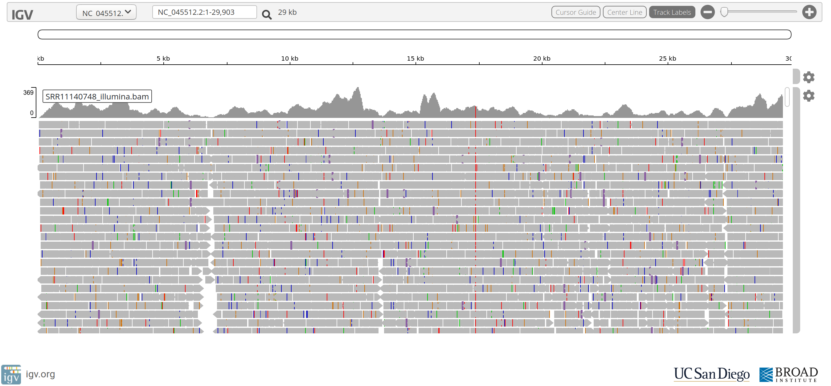
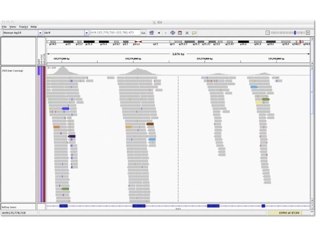
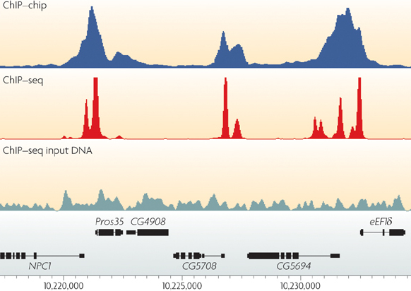
One of the most fundamental aspects of genomics applications is visualising what an alignment looks like. The stacks of reads that align to certain positions on the genome, or what Bioinformatician’s call “pile-ups”, are a very important quality control aspect of the sequencing process. By viewing the alignments and visalising the “coverage” of specific areas of the reference, you are able to diagnose events that happened during data processing. Each genomics application, whether it be Whole Genome Shotgun (WGS) sequencing, RNA sequencing, or targeted approaches such as ChIP-seq or Exome sequencing, has a characteristic alignment pattern.
For example, lets look at some coverage figures taken from recent publications or websites that display the coverage for that particular genomics application:
- RNA-seq

- WGS
- Exome sequencing
- ChIP-seq
Task
- Describe the coverage that is displayed in each of the above figures and discuss the technical and/or biological functions that govern them
- i.e. why does the coverage look the way it does?
How do we look at our alignment?
To round off the tutorial, lets have a look at our file using a genome browser.
Generally the easiest way to view a alignment file from a model organism such as human or mouse it to use a program such as IGV or UCSC Genome Browser, which also contain a number of handy utilities to look at genes and regulatory features.
However because of the constraints of our VMs, today we’re going to use one of the most basic alignment viewers that is included in samtools.
I generally use this alot for a quick look, and it can be a really handy way of initially visualising reads.
Using the reference sequence that was included in the data downloaded today, lets use the samtools tview subcommand: (for this to work, we need to have a decompressed reference genome)
#We use pigz to decompress rather than gunzip as it uses all available cores
pigz -d ./data/GRCh37.p13.genome.fa.gz
#Need to make the index for the bam file
samtools index ./data/SRR3096662_Aligned.out.sort.bam
#initiate tview
samtools tview ./data/SRR3096662_Aligned.out.sort.bam --reference ./data/GRCh37.p13.genome.fa
Looks like nothing now, but the first part of the chromosome should not have any coverage at all. Lets try looking for coverage over a gene like CGB1. Press “g” on the keyboard and type in “chr19:49538826”. This means chromosome 19 and position “49538826”.
Spend some time looking across this gene and see what features you can make out.
For example, do you see any occasions where a nucleotide is different from the reference?
When you are done, type “q” to quit the tview tool.